In short. On its own, the oscillator network did not learn to recall a value by its key, and neither did the standard models we compared it with. Given the same lookup mechanism as its competitors, it reached 94.3% on a 32-step memory task and 72.0% on a harder 64-step one: well ahead of a state-space model (88.2% and 53.5%) and slightly behind a GRU (96.1% and 76.5%) that had about 50% more trainable parameters. Three seeds and one synthetic task are not enough to call this an advantage. The simulation is also far slower than the alternatives. The idea is not ruled out, and it is not proven.
The question
Most AI models keep track of the past with layers of numbers that are updated step by step. We wanted to know whether a different kind of system could do part of that job: a network of oscillators, each with an amplitude, a phase and a frequency, that influence one another. Physical systems of this kind exist in optics and electronics, which is why the idea is interesting. Before anything physical makes sense, though, the idea has to work as mathematics.
We wrote the question down before running anything, in a design approved on 2 September 2026:
With the same budget of state, memory and training, does the wave dynamics give a reproducible advantage over comparable recurrent networks and feature maps?
The design also fixed three hypotheses: that oscillators can learn tasks needing both memory and non-linear processing; that phase, coupling and non-linearity each contribute, rather than the result coming from more features or a bigger readout; and that performance improves predictably with more oscillators. A fourth, that physical hardware could run this more cheaply, was explicitly set aside: a software simulation cannot test it.
The model and the comparisons
The “Wave” model is a network of Stuart–Landau oscillators. Each oscillator z is a complex number that evolves as dz/dt = (μ + iω − β|z|²)·z + Σ K·z + B·u(t): a natural frequency ω, damping and saturation (μ, β), coupling to the other oscillators K, and the input u. The equations are integrated with a fourth-order Runge–Kutta method, 20 sub-steps per input.
Every probe compared it against the same alternatives, under the same data, splits, seeds and training budget:
- Standard recurrent models: a GRU, a complex diagonal state-space model (SSM) and an echo state network (ESN).
- Wave with parts removed: no coupling, no non-linearity, or amplitude only, to see which ingredient matters.
- Floors and ceilings: a model that sees no history at all (it should score at chance) and an explicit memory or exact lookup (it should score near 100%). If either misbehaves, the test itself is broken.
- Simple rules: for example, “always answer the most recently written value”, which a model has to beat before its score means anything.
Conditions
| Hardware | One Windows 11 desktop PC. Most scientific runs on the CPU, on a single thread; the last diagnostics on an AMD Radeon RX 7800 XT. |
|---|---|
| Software | Python 3.12 and PyTorch 2.13, with locked dependencies. Ruff and 239 automated tests passed before the pilot; an 88-cell smoke run completed without failures. |
| Tasks | Delayed XOR and NARMA-10 for the pilot; then a synthetic memory task: several keys are written with values, interrupted by distractors and corrections, and a final question asks for the value of one key. The answer is picked from four candidates in random order, so chance is 25%. Every label is checked by an exact algorithm; no AI model was used to grade answers. |
| Seeds | 7, 19 and 31, fixed in advance. A failed seed is not replaced. |
| Fairness | Same state width for every model (16, later 128 numbers), same readout and scorer, same learning rate, update cap, evaluation cadence and gradient clipping. Parameter counts are reported, because they are not equal. |
| Test sets | Generated from fresh cryptographic seeds only after every checkpoint was sealed and hashed. Checkpoints are chosen on validation loss, never on the test. |
The pilot that stopped itself
The planned pilot had 180 cells. Before training anything, it measured its own cost. Training the oscillator network with 16 oscillators took 3.75 seconds per update on the CPU, which projected the whole pilot at about 65 hours against a preregistered limit of 8. The gate stopped it after six completed cells, and the report was labelled Insufficient evidence, as every smoke and pilot run is by rule. Before the pilot, a target-free diagnostic also showed that the original oscillator settings were too narrow in phase and too close to linear; they were amended without looking at any task result.
We then switched to shorter, capped probes on the memory task, each with its own stopping rules.
Probe 1: fixed oscillators, 1 October
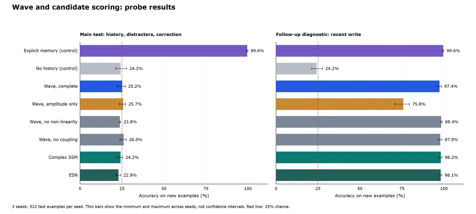
First, the oscillators were left untrained (only the scorer reading their state learned), as in classic reservoir computing. 48 cells ran in 3.6 minutes.
Dashed line: chance (25%). Eight oscillators, three seeds, 512 test examples per seed. The explicit memory is a positive control with a different architecture, not a fair competitor.
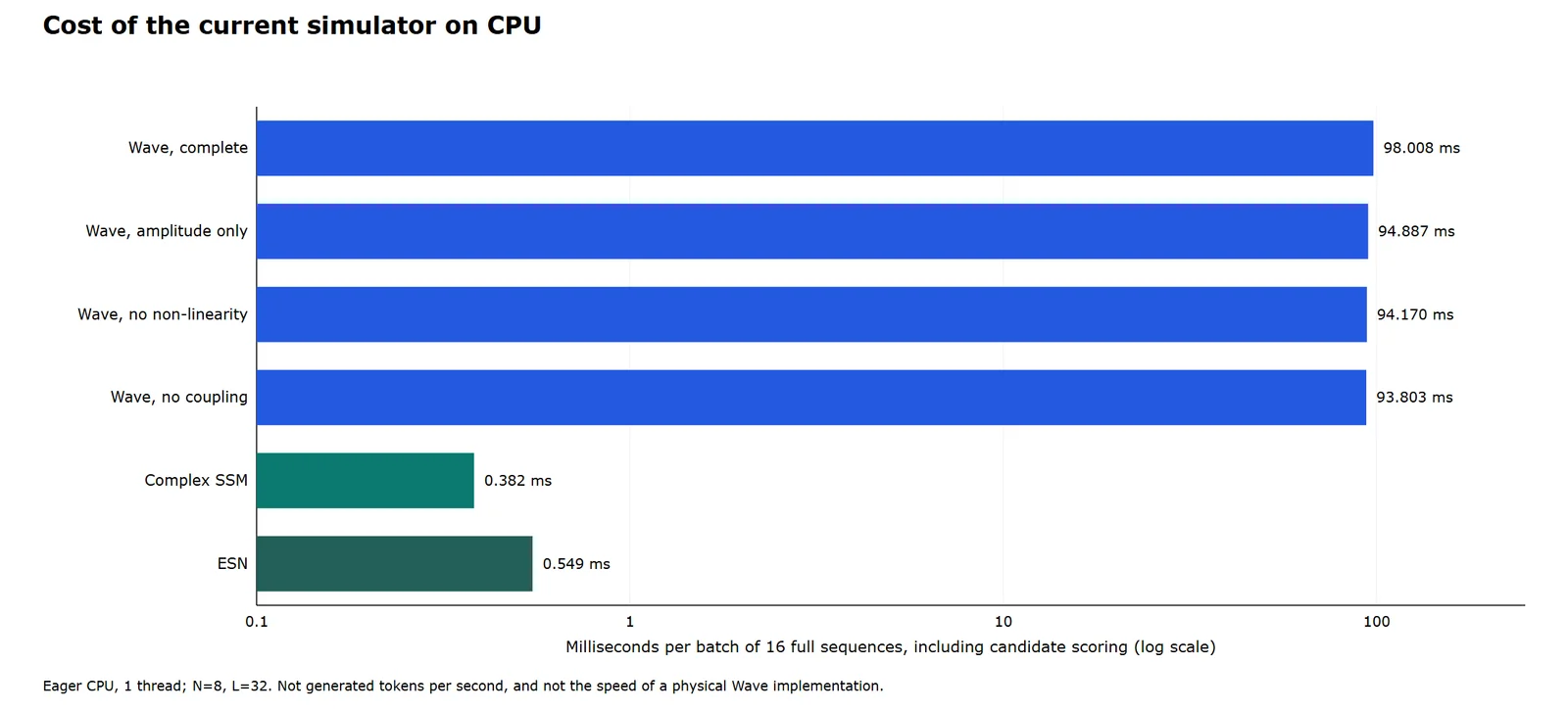
Every untrained model stayed at chance on the real memory test. On an easier diagnostic, recalling the value written just before the question, all of them reached 97–99%, so the pipeline worked; the long-range memory did not. Removing phase (amplitude only) clearly hurt, but removing coupling or non-linearity did not, so this probe showed no ingredient that is unique to Wave. It was also about 256 times slower than the SSM in our simulator: 98 ms against 0.38 ms per batch.
Probes 2 and 3: training the oscillators
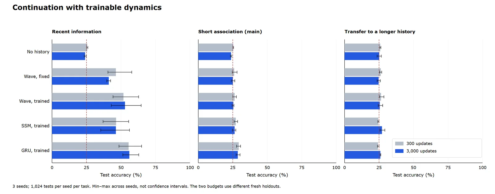
Next we trained the oscillator dynamics themselves, against a trainable SSM and GRU, first on a fixed dataset and then with fresh examples at every step: 31,200 distinct episodes per seed.
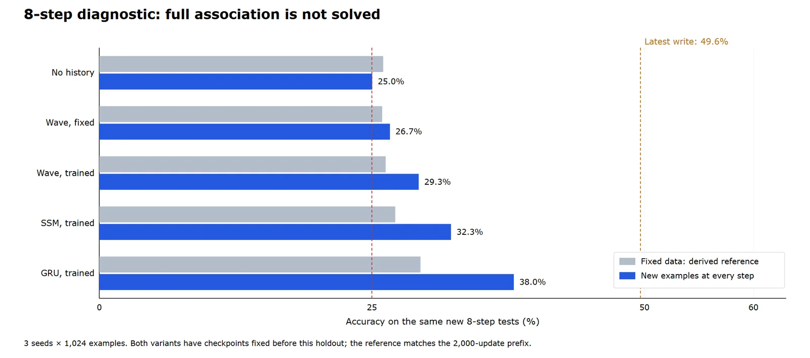
Chance. “Latest value” rule (49.6%). Three seeds × 1,024 test examples. Checkpoints were sealed before the test set was generated.
Training helped a little, but no model beat the trivial rule of answering the latest value (49.6%). When we kept the history and changed only the key being asked, the GRU changed its answer in about 8.7% of cases, although the correct answer always changed. Its higher score reflected remembering recent values, not looking things up by key. On the 32-step version of the test, scores fell to 25–31%. An earlier version of this report did not show the 32-step results prominently enough; we corrected it after review.
Probes 4 to 6: a shared lookup mechanism, 2 October
Training and testing directly on 32 steps, all three models still stayed at 25% when the answer had to come from their final state, while a control with built-in key lookup reached 98.2%. So the bottleneck was reading the memory, for every architecture. We then gave all three the same trainable query–key readout, which looks over their state at each step. This is what produced the results we find most interesting.
Chance. Three seeds; 24,000 distinct training episodes per seed. The 64-step task has 8 keys, each written twice, and 47 distractors. At 64 steps the control trained for 1,500 updates and the three models for 800, so its score is a reference, not a like-for-like comparison.
On the harder 64-step task, Wave was 18.5 points ahead of the SSM and 4.5 points behind the GRU. Counting only trainable parameters, as corrected by the independent review, Wave used 2,091, the SSM 1,955 and the GRU 3,155: about 34% fewer than the GRU. On questions where both the original and a swapped key had to be answered correctly, Wave scored 60.2%, the SSM 35.6% and the GRU 65.1%.
Two attempts at the 64-step task were stopped before any model was compared, because the lookup control did not pass its own gate (78.1% against a required 80%). A test that even its ceiling cannot pass says nothing about the models, so we did not report one.
One limit matters here. The shared readout looks at the state of every step, not only the final state. This shows how well each model works with external lookup over its history; it does not show that the oscillators compressed eight associations into their final state.
Probe 7: memory inside the final state
The last round asked the harder question: can a model build that memory inside a final state of 128 numbers? Our rule was that the GRU, the strongest standard model, had to pass first. It did not (26.6% and 25.0% with two learning rates), so Wave and the SSM were not compared. Diagnostics then showed why. A learned scorer reading a perfect, hand-built memory still reached only 38.6% on new examples, while an explicit key-matching reader reached 100%. With that explicit reader, a GRU trained through a curriculum from 2 to 8 keys still stayed at chance on 8 keys over 64 steps. We stopped there, as the protocol required.
What we found
- Oscillators are not a shortcut to memory. Untrained, or read only from their final state, they did no better than chance at recalling by key. Neither did the GRU or the SSM under the same conditions.
- With the same lookup mechanism, Wave was competitive. It beat the SSM by a wide margin and came within a few points of a GRU that had about 50% more trainable parameters. That is a signal worth testing again, not a demonstrated advantage.
- The hard part is writing and reading memory, for every architecture. Most of the failures were shared by all models, which points to the recipe and the readout rather than to Wave itself.
- The simulation is expensive. On a CPU, simulated oscillators were around 256 times slower than the SSM. Whether physical oscillators could be cheaper is a separate question this work cannot answer.
- The stopping rules worked. The pilot, two 64-step runs and the final-state comparison were all stopped by gates set in advance, before they could spend compute on results that would not mean anything.
How we kept ourselves honest
- The question, hypotheses, fairness rules and verdict labels were written before the first run. The one change before the pilot was recorded as an amendment, made without looking at any task result. The later probes were exploratory, and each report says so.
- Every run records its configuration hash, source fingerprint and checkpoint hashes. Results are never overwritten.
- Test sets were generated only after checkpoints were sealed, and checked for overlap with training, validation and gate sets.
- Two independent reviews re-checked the first probe and the 64-step comparison. They reproduced the reported accuracies from the saved predictions and checkpoints, found no label leakage or duplicate episodes between splits, and corrected one error in how we counted parameters. We published the correction and kept the original logs.
- Every verdict so far is Insufficient evidence or inconclusive. That is the honest label for three seeds and one synthetic task.
What we do not claim
This was a numerical experiment on synthetic tasks, not a language model. It does not measure text generation, general ability, tokens per second or energy use, and nothing here shows that oscillator hardware would be faster or more efficient. A negative result in these configurations does not rule out every oscillator architecture, and the positive signal does not establish superiority.
The work is paused. If we continue, the next comparisons are already defined: a simple encoder without any recurrence under the same readout, Wave with coupling, phase or non-linearity removed under that readout, and more seeds and tasks. We will publish those results here, whichever way they go.
Charts from the lab
The lab’s own charts for the first three probes, redrawn in English from the same result files. Select a chart to open it at full size.
The data
Every number on this page, model by model and probe by probe, is in one file you can download and check: wave-ai-results.csv (CSV, 75 rows). Values are averages over seeds 7, 19 and 31, as reported by the lab after each probe.
Radovar is the software company behind Codevalanche, a desktop app for coding with AI agents. This research is separate from the product and does not describe how Codevalanche works.
More research: all articles. Questions about this work: info@radovar.com. More from us on the Updates page.